LogViewer tab
Substrate management tabs
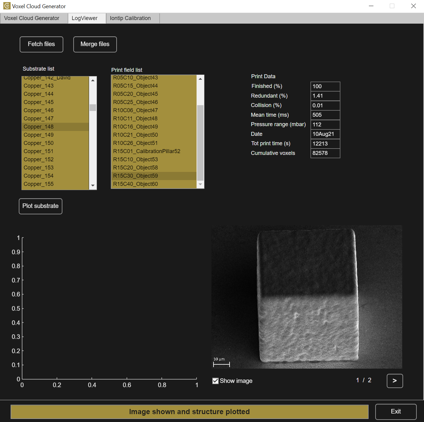
Located in the top left quarter of the LogViewer tab, one list selects a substrate and a second list any of the objects printed on the selected substrate. When a printed object is selected, a Printed Object figure opens with each voxel (color-coded) that is contained in the file. Additionally, selected printing statistics are displayed in the top right quaroter of the tab.
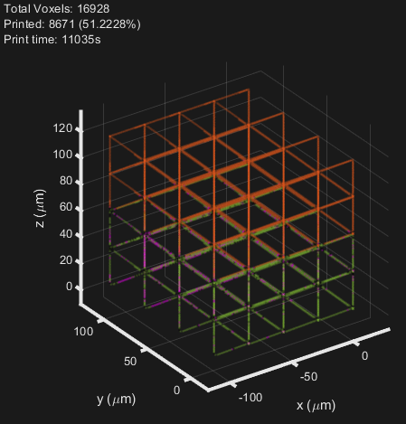
The color code is the following:
- regular voxel : the detection triggered after the approach to the voxel position
- missing voxel : the voxel was not printed, the printing stopped before reaching this voxel
- collision voxel : detection triggered while moving to the XY voxel position
- redundant voxel : detection happened while approaching the voxel Z level after reaching its XY position
Available interaction with the figure:
- rotate (left click dragging in the figure)
- zoom (wheel)
- pan along one axis (left click on the selected axis and drag)
- restore default view (house icon)
- datatips (left click on a voxel with the datatip icon toggled)
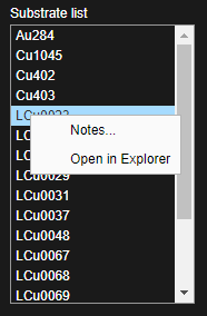
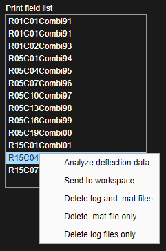
Log files can be gathered and analyzed to generate a report file (.mat). This file is then used to plot data, graphs and statistics on the objects printed. To access those options right click on a substrate or on objects to open the respective contextual menus.
Buttons functions:
-
Fetch files: Move and sort the log files available from the<BaseExportDirectory>to the database in their respective substrate folders. -
Merge files: Merge the 5 different log files of each object of the selected substrate and generate the .mat report file. Once merged, an object file is displayed in the print field list and is also accessible by the VCG tab (substrate plots, collision detection,…). Merging is also a necessary step for theIontip Calibrationprocedure. -
Plot Substrate: Display an overview of the selected substrate in the bottom left figure based on the .mat report files available.
The contextual menu options for the substrates list are:
-
Notes: Open the Notes dialog or create a note files for the selected substrate. This can be used to write or read additional information about this substrate. -
Open in Explorer: Open the substrate folder in Windows explorer.
Structures contextual menu options are :
-
Analyze deflection data: Display different curves showing the recorded data during printing. -
Send to workspace: Load the report file in the MATLAB workspace for manual access and analysis. -
Delete .log and .mat files: Delete all log and report files related to the selected object. Deletes the object and all its information from disk. -
Delete .mat file only: Only the merged .mat report file of the selected object is deleted. The .mat files is recreated by clicking theMergebutton. -
Delete .log file only: Only the log files are deleted. All the information on the object is still accessible in the .mat report file. This is a useful function to save disk space.
Print data
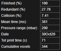
The print data table summarize the key values related to the selected object.
Note
The pressure range indicates 1 value when pressure is the same for all voxels, and the [min max] range when different values were defined in the printfile.
Plot Substrate
The bottom left figure shows the selected substrate overview created with Plot Substrate. All merged .mat files available are used to plot the structures in gold viewed from the top. Row and column labels are added to identify each object on the substrate.
Transformations added in CAPA are also included in the preview via the PL log file.
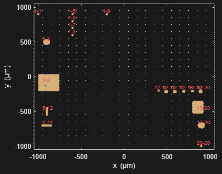
Holding the left click and dragging draws a zooming box around the area of interest. Plot Substrate can be used to reset the view.
Show image
The LogViewer can display images that are taken of each printed object (in SEM or optical microscope for example). To use this feature observe the following instructions with case-sensitivity.
- Select the relevant substrate and use
Open in Explorer. - Create a folder called
imageand copy the images of the object in this folder. - Images must be named
SubstrateName_r[Row Number]c[ColumnNumber][_suffix] to fit their imaged object name. The suffix can be anything to differentiate multiple images of the same object. Row and column numbers must be in a two-digits format (01-99).
Example
If the substrate name is Sub1 and the row is 1 and the column is 5, the image name is Sub1_r01c05, placed in a folder ./analysis/Sub1/image.
If there are multiple images taken of the same print field, add an underscore and a suffix. The extension of the image should not be changed. Any image supported by the MATLAB function imshow will be shown in the GUI. Folder and file names are case sensitive.
The LogViewer only displays images if the checkbox Show image is checked, a
print field is actively selected in the print field list and that object has images properly named (two-digits format, case sensitive, etc.). If multiple images are associated with the same print field, the first image will be displayed
and a > icon will appear to go to next image and move through all images.